Variability of Additive Manufacturing Processes Part 2

Part One of this series by Todd Grimm can be found here.

Table 2, which is generally ordered by best to worst COVs, presents the values used for Figure 2. FDM had the lowest COVs for tensile modulus (1.84% and 2.51%) and EAB (4.96% and 11.54%) in both coupon orientations. For tensile strength, FDM had good COVs (2.13% and 3.37%), which were within 1.38 percentage points (PP) of the best results. MJF’s COVs for tensile strength and tensile modulus ranged from 1.05% to 4.01%. SLA had similar results with COVs ranging from 1.82% to 3.55%. Excluding MJF’s COV for EAB in the XY orientation (21.05%), both MJF and SLA had good COVs, ranging from 9.15% to 14.12%, for elongation. For tensile strength and tensile modulus, SLS’s and CLIP’s COVs ranged between 5.77% and 16.09%. While CLIP had a lower COV for tensile strength (9.02%), SLS had much better tensile modulus values (5.77% to 6.07%). Both processes also had high to very high EAB COVs, ranging from 22.09% to 44.88%. FFF performed well with tensile strength in the XY orientation (5.95%), but it had poor consistency in all other measures with COVs ranging from 14.08% to 54.06%. While standard deviation (SD), mean values and data ranges are not suitable for comparison, as described previously, these results are shown in Figures 3, 4 and 5 to provide a visual representation of the individual tests results that contributed to the COV values. Plotting each measured value provides visual representation of the dispersion of results. For example, FDM’s tensile strength (XY) and MJF’s EAB (XY) were influenced by a few outlying values.

Machine to Machine

Historically, AM processes have demonstrated build-tobuild and machine-to-machine variances. To determine the influence of machine-to-machine variances on COV, Figures 6, 7 and 8 show the percentage point differences between the two machines used to build the tensile test coupons for each process. A small range is desirable since it indicates repeatability in outputting parts with little variation in mechanical properties across multiple machines. In these charts, the range boxes’ upper limits are the highest COV from the two machines. The lower limit represents the COV for the other machine. For example, FDM’s combined COV for tensile strength (XY) was 3.37%. Figure 6 shows that the COVs for the FDM machines were 1.63% and 4.23%, which is a small 2.6 percentage point (PP) difference. Tensile strength is shown in Figure 6. It reveals that FDM, MJF, SLA and CLIP had both a low overall COV and a low variance between the machines. Collectively, the differences between Machine 1 and Machine 2 are small, ranging from 0.37 to 2.60 PP. Therefore, these processes should be expected to produce consistent results across multiple machines.

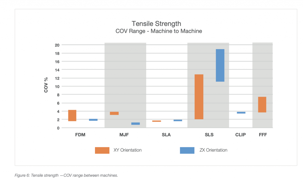
FFF, in the XY orientation, had slightly larger machineto-machine variance with a 3.84 PP difference. Since no test coupons were made on a second machine, due to the previously described issue with building in the ZX orientation, FFF had no comparative results for that orientation. SLS yielded the highest machine-to-machine variances, with 10.83 PP and 7.8 PP for XY and ZX, respectively. Interestingly, SLS Machine 1 had a very low COV for XY coupons while Machine 2 had a low COV for ZX samples. Figure 7 plots the COV range boxes for tensile modulus. The results for FDM, MJF and SLA were very similar to those for tensile strength. SLS, CLIP and FFF, on the other hand, showed pronounced differences. SLS proved to be more consistent for tensile modulus with COV ranges of 5.03 PP (XY) and 2.28 (ZX). Both CLIP and FFF had greater variances when compared to tensile strengths. CLIP had a difference of 5.77 PP, and FFF had a difference of 10.55 PP.

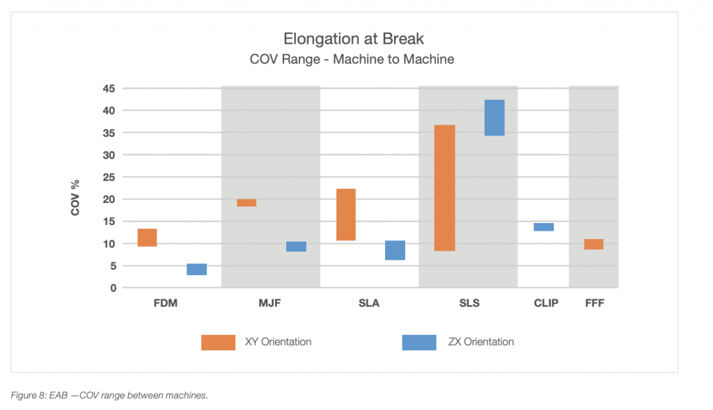
The last machine-to-machine comparison is for EAB, which is shown in Figure 8. FDM, MJF, CLIP and FFF all had small variances between machines with values ranging from 1.57 PP to 4.07 PP. While the ZX value for SLA was also good, the XY difference between machines grew to 11.96 PP. SLS’s XY difference was the largest of any machine-to-machine variance for all properties with a 28.60 PP difference.

This series was written by 3D Printing Consultant Todd Grimm, with the support of Stratasys.